MLP from Scratch: Fashion-MNIST

Overview

The goal of this post is two-fold:

1. To provide additional context and highlight some essential parts from the MLP.ipynb Jupyter notebook in the Github repo for the project
2. To selfishly serve as a refresher to basic ideas behind layers and backpropagation seen in popular ML libraries like PyTorch.

With that in mind and to keep it brief, I will assume some knowledge of what an MLP is and non-linear activations such as the Softmax function, matrix multiplication, etc.

Getting started

The data

For this project, our task is multi-class classification using the Fashion-MNIST dataset, which consists of 28x28 px monochromatic images labelled into one of 10 different clothing item categories.

Pre-processing the data

Each pixel value in an image is an integer ranging from 0 - 255. In this case, the scale of features is bounded and approximately the same, so it is unnecessary to do something like z-normalization, where we subtract the mean and divide by the standard deviation. However, dividing the images by 255 (i.e. scaling the range between 0-1) sped up the training process and achieved a more stable conversion.

Flattening & One-hot encoding

One-hot encoding converts categorical labels like (0, 1, 2, 3,…) for the different clothing items into vectors with length equal to the number of classes. In this vector, the index equal to the categorical label would have a value of 1, with all other indices being 0. This allows the network's output layer to represent each class's probability independently.

We flatten the 2D images into a vector, which is the required input format for our MLP since we do not have a sliding window approach as in a CNN. Here, flattened_train_images is a 2D array where every row represents a flattened image from the original train_images set:

flattened_train_images = np.array([train_images[i,:,:].flatten() for i in range(len(train_images))])

Building the MLP

NeuralNetLayer

This is the basis for the layers we will compose into our MLP. In an informal sense, it behaves like an abstract class because it is designed to be subclassed. It contains two instance attributes, .gradient and .parameters.

class NeuralNetLayer:
    def __init__(self):
        self.gradient = None
        self.parameters = None

    def forward(self, x):
        raise NotImplementedError

    def backward(self, gradient):
        raise NotImplementedError

Linear Layer

This is a subclass of the NeuralNetLayer, and it implements the forward and backward passes of the layer.

The Forward Pass

In the forward pass, we compute the linear transformation Wx + b. The trick here is that we are using Python broadcasting for this operation. Let's take a look at what that looks like:

• self.w[None, :, :] has shape (1, output_size, input_size)
• x[:, :, None] has shape (batch_size, input_size, 1)
• self.b has shape (output_size,)

Due to broadcasting, the operation self.w[None, :, :] @ x[:, :, None] performs batch matrix multiplication between the shapes of (batch_size, output_size, input_size) and (batch_size, input_size, 1). In this way, you have 'batch_size' many matrices of size (output_size, input_size) being multiplied by 'batch_size' many matrices of size (input_size, 1). Following matrix multiplication rules gives us an output shape of (batch_size, output_size, 1). We then squeeze this to remove the last dimension, leaving us with (batch_size, output_size) for the result of multiplication of the weights with the input.

The Backward Pass

The goal here is: given the gradients received from the subsequent layer, calculate the gradients relevant to the current layer's parameters (when applicable) and determine the gradients to be forwarded to the preceding layer.

Therefore, for the backpropagation of our MLP, we start with calling backward on the output label and then preceding layers (using the output from the subsequent layer as input) until we reach the first layer. This recursiveness in the chain rule update can be seen in the slide courtesy of Prof. Yue Li (COMP551, Fall 2022):

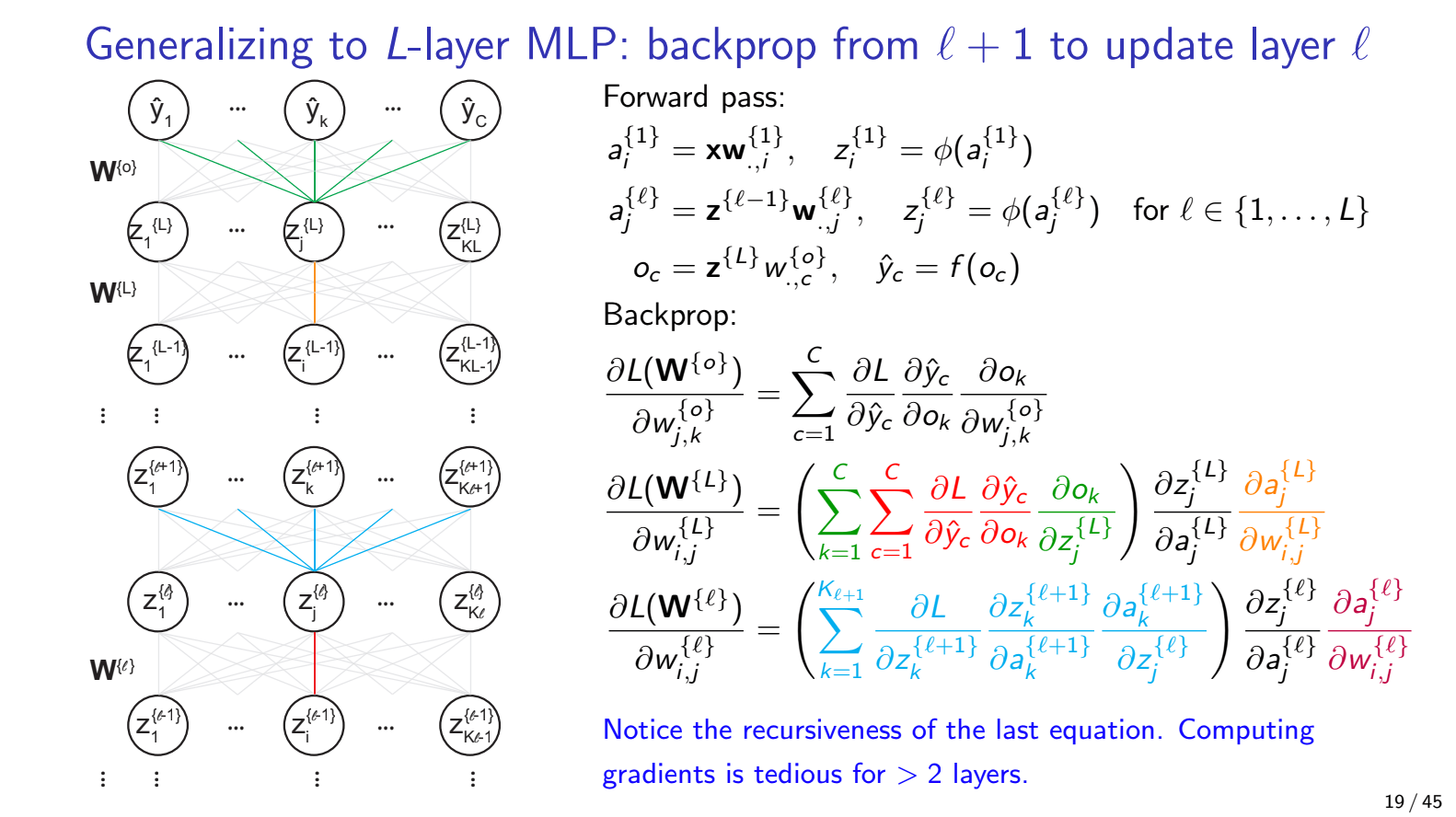
In the backward function, we calculate the gradient w.r.t the weights dw and the bias b and return the gradient w.r.t the input.

def backward(self, gradient):
        assert self.cur_input is not None, "Must call forward before backward"
        #dw = gradient.dot(self.cur_input)
        dw = gradient[:, :, None] @ self.cur_input[:, None, :]
        db = gradient
        self.gradient = [dw, db]
        return gradient.dot(self.w)

To see how we get the statement we're returning, consider

$ \textbf{z}^{\text{{2}}} = \phi(\textbf{a}^{\text{{2}}}) $ which is the post-activated output of layer one or input at layer two and $ \textbf{a}^{\text{{2}}} = \textbf{z}^{\text{{1}}}\textbf{W}^{\text{{2}}} $ which is the pre-activated output of layer 1. By the chain rule, we have:

\( \frac{\partial \textbf{z}^{\text{{2}}}}{\partial \textbf{z}^{\text{{1}}}} = \frac{\partial \textbf{z}^{\text{{2}}}}{\partial \textbf{a}^{\text{{2}}}}\frac{\partial \textbf{a}^{\text{{2}}}}{\partial \textbf{z}^{\text{{1}}}} \)

$ \frac{\partial \textbf{z}^{\text{{2}}}}{\partial \textbf{a}^{\text{{2}}}} $ is the from the subsequent layer and is stored in self.gradient. Therefore, we need to determine $ \frac{\partial \textbf{a}^{\text{{2}}}}{\partial \textbf{z}^{\text{{1}}}} $ which is just the weight matrix $\textbf{W}^{\text{{2}}}$ and that is why we return the dot product of the gradient from the preceding layer with the weight matrix of the current layer.

If you want a more in-depth look at the math, I recommend this article.

Other layers & SoftmaxOutputLayer

The other layers implemented here are activation functions whose forward and backward methods are more straightforward. However, I would like to call attention to the SoftmaxOutputLayer.

In this case, the forwards method is simply the Softmax function; however, since we are using the Cross-Entropy loss function for multi-class classification and are only using the softmax on the output, we combine the gradient of the loss and softmax.

\( \frac{\partial \mathcal{L}(s, y)}{\partial x} = s - y \)

Where $s$ is the logits output from the softmax function for input $x$, $\mathcal{L}$ is the Cross-Entropy loss, and $y$ is the array of one-hot encoded labels. For the complete derivation of this, here is a great reference.

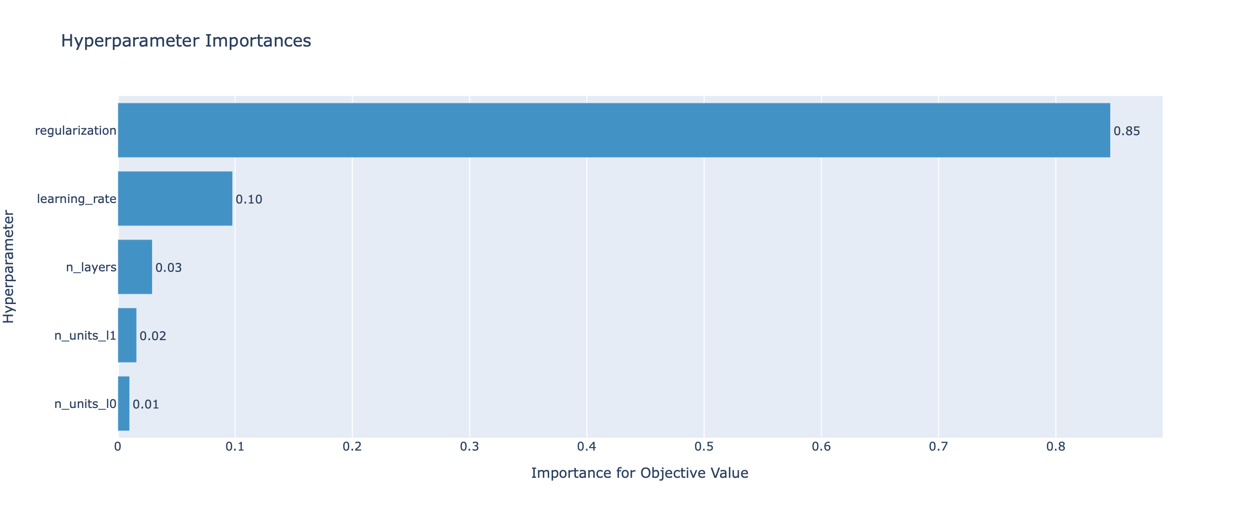
Hyperparameter Tuning

The library Optuna was used for hyperparameter tuning.

Here, we tuned several parameters, including the number of hidden layers, the width of the hidden layers, the learning rate and the weight decay. In the case of vanilla SGD, weight decay is the same as L2 regularization (more on that here).

The importance of hyperparameter tuning is well-illustrated in the notebook, as we observed a roughly 9% increase in validation accuracy after tuning. Another great thing about the Optuna library is that it offers ways to visualize the relative importance of the hyperparameters for the objective metric like so:

Summary

• We discussed the concepts behind data pre-processing
• Overviewed the NeuralNetLayer and LinearLayer classes, which are the building blocks for our MLP
• Looked at the relative importance of hyperparameters

Thanks for reading!